The Backyard Brains 2018 Summer Research Fellowship is coming to a close, but not before we get some real-world scientific experience in! Our research fellows are nearing the end of their residency at the Backyard Brains lab, and they are about to begin their tenure as neuroscience advocates and Backyard Brains ambassadors. The fellows dropped in […]

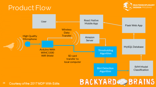Hello friends, this is Yifan again. As the end of the summer draws near, my summer research is also coming to a conclusion. The work I did over the summer was very different from what I expected. Since this is a wrap up post for an ongoing project, let us first go through what exactly […]

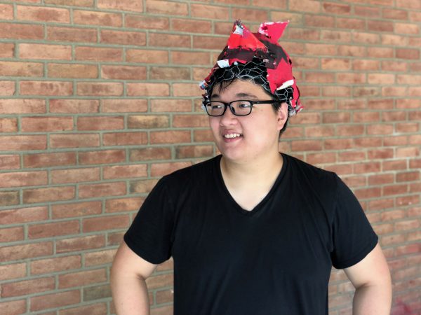Hello again everyone! It’s Yifan here with the songbird project. Like my other colleagues I also attended the 4th of July parade in Ann Arbor, which was very fun. I made a very rugged cardinal helmet which looks like a rooster hat, but I guess rooster also counts as a kind of bird, so that […]

One of the most attractive things about a BYB Summer Fellowship is the chance to spend a summer in colorful Ann Arbor. We changed the program name from an internship to a fellowship because of the lasting connections made throughout the summer, and these connections are made possible by the things we all do together! […]

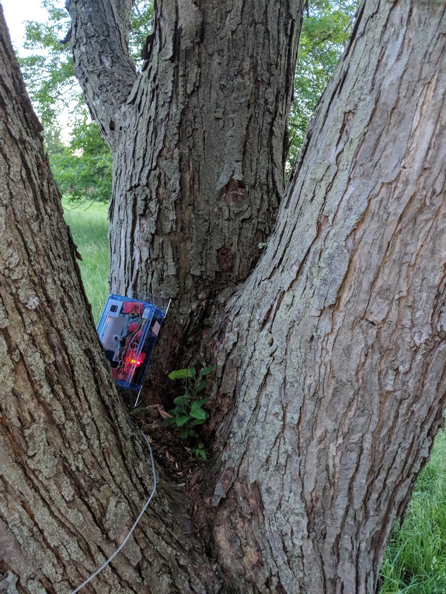Hey guys, it’s Yifan again. There has been a lot of progress since my first blog post. As promised last time, I was able to finish a functional prototype with all the legacies left for me. I put the device in the woods to get recording for the first time. The results, to my pleasant […]

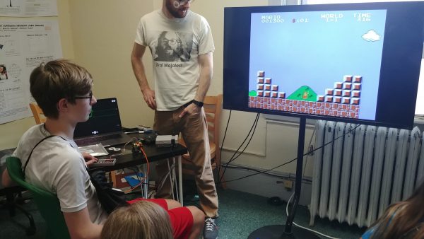Fresh, organic, locally sourced meditation researchLast Friday, Backyard Brains once again opened our doors (even wider–they’re always open during business hours!) to our fellow and aspiring citizen scientists as a part of this year’s Ann Arbor Tech Trek!  Dozens of local tech companies had their doors open to the public that evening and we, like […]

Hi I’m Yifan, a senior studying Computer Science at University of Michigan. I’m working on the Rainforest Wildlife Recording Project. This project is a continuation of 2017 fellow Zach’s Songbird program. Me and my teammates also worked on this during last semester, and will continue to improve it in the coming semester. We have already […]

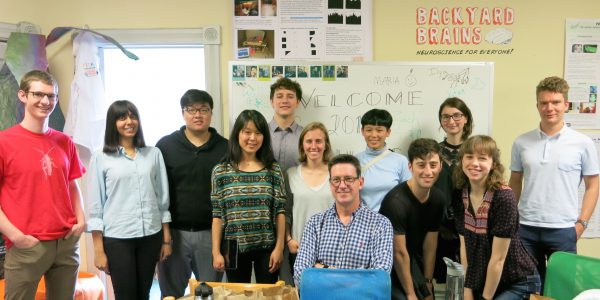From left: Ben, Anusha, Yifan, Jessica, Aaron, Jess, Greg Gage (not a Fellow), Maria, Dan, Anastasiya, Molly, Ilya Meet the Fellows, See the Projects The fellows are off to a great start! This week has been focused on them getting their feet wet with our kits and learning about what we do here at Backyard Brains. Be […]

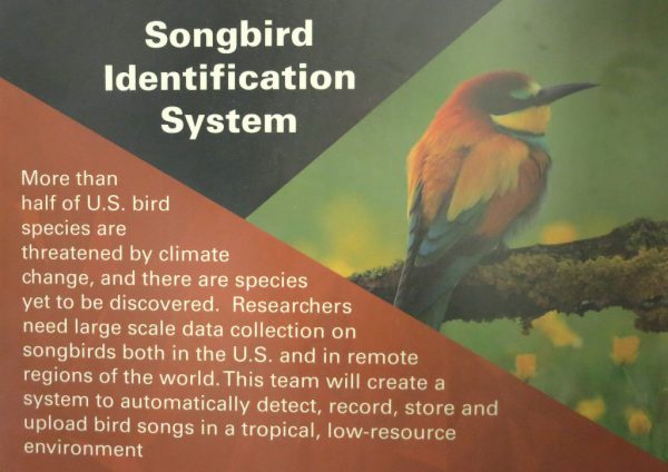Acoustic Wildlife Recording promotes Citizen Science! Here at Backyard Brains, we are all about citizen science, or the idea that the scientific community benefits from the collaboration with members of the general public for collecting and analyzing information about the natural world. Very DIY, very much the “for everyone” in our slogan. In 2017, Backyard Brains […]

Hey, Zach here with another songbird identifier update! Since the last post, I have been busy testing the prototype device by taking bird recordings in various locations. After this week I will be taking a short break before resuming work on the project with the rest of the songbird team in the coming semester. Right […]

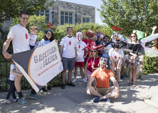Over 11 sunny Ann Arbor weeks, our research fellows worked hard to answer their research questions. They developed novel methodologies, programmed complex computer vision and data processing systems, and compiled their experimental data for poster, and perhaps even journal, publication. But, alas and alack… all good things must come to an end. Fortunately, in research, […]

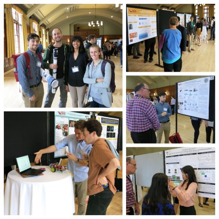
Today our Summer Research Fellows “snuck in” and presented their summer work at a University of Michigan, Undergraduate Research Opportunity Program (UROP) symposium! Over the two sessions our fellows presented their work and rigs to judges, other students, to university faculty, and community members. Some of the fellows are seasoned poster designers, but others had […]